Synopsis:
=Vlookup(what you are looking for, where, which column, exact-match=False)
or
=IfError(Vlookup(what, where, column, false),"Not Found")
Summary of steps:
1. In a separate sheet, create table of values to lookup
2. Range-name the lookup table (minus header row)
3. Build VLookup, selecting base-1 column name
Contents:
- VLookup - Name the Range
- Parameters
- Selecting the Range - the "trick"
- Improved VLookup using IfError
- Fixing Range Names
- Performance Concerns
- Dirty (Numeric) Data
- Non-exact searches (within a range of values)
VLookup Introduction:
In Excel, a VLookup allows your sheet to lookup another value from another sheet, cross-referencing catalog information into the current sheet.
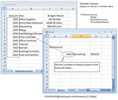
For example, a Master Account number table could show a description, budget numbers and the person in-charge of that account. Then, in any number of other sheets, you can lookup the account number and return those centralized values into the current workbook:
 |
| Click for a larger view |
In other words, your sheet could reference an Account number (illustrated, in Cell B5), and multiple other values from the lookup table, such as the description and budget-amounts, can be returned in a cross-lookup.
If data in the lookup table changes, for example, assume the dollar'd budget amount changes, the new sheet picks up the new value automatically. With this, one group of people can maintain the account list, and all other linked sheets will see the most current values.
VLookup Setup:
Build an Account Number Master list.
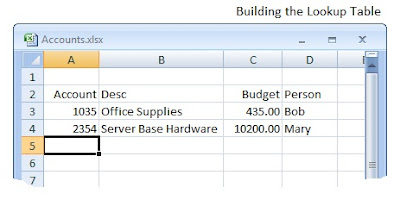
In a (usually) separate sheet, make a list of values to lookup, with the Account number as the first column. This can be account codes, employee numbers, part-numbers, people names, etc.
1. Open a new, blank spreadsheet.
2. Load or type account information, where:
- The first column must contain a unique value (the Key) for each record.
This is the Account Number - No duplicate entries are allowed in the first column.
- Any number of columns can follow the first (Description, budget, etc.)
- Column headings are recommended, but not required.
- The list *must* be sorted alphabetically/Numerically by the first column. (Technically, it 'should be' sorted if you are using "exact-matching"; it 'must' be sorted if not exact-matching. Sorting is always recommended.)
Name the Range:
Although optional, I recommend naming the data-range. Follow these steps:
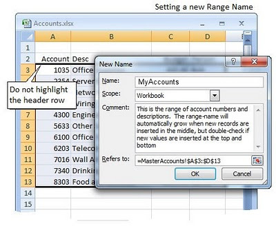
3. Once the lookup values are typed, highlight the data (all rows, all columns, *not including* the Header row)
a. 'Other-mouse-click' the highlighted cells, choose "Name a Range"; name the range a meaningful name, such as "MyAccounts". No spaces.
a2. (Alternately: Click top Menu Formulas, Define Name and type the range, using dollar-signs to lock the rows and columns. For example: $A$3:$D$13)
a3. (Another alternate method): Highlight the data, minus the column headers, then click in the area directly above column A. Type the range-name there.
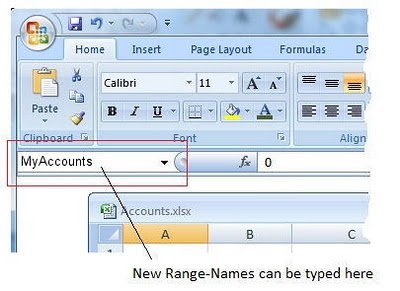
The Range-name makes future work easier, see below for more information.
b. Save the entire sheet to disk, giving it a meaningful name such as "Accounts.xlsx" or "FY17Accounts", etc.
Once saved, leave the sheet open while building the Vlookup formulas. In the future, this sheet can be opened or closed and it will still work properly -- but if already opened, lookups are faster.
Using VLookups in your Sheet
4. In a new sheet (File, New, Blank workbook), where you want the results to appear, move to an arbitrary cell (B5).
5. Literally, type an account-number to look up: For example, "2356"
 |
| Click for a larger view |
Note the popup help:
a. For the first parameter, after the parenthesis, click cell B5 (2356). This is the value you are trying to look up.
* Type a Comma (,) to move to the next parameter.
b. While still in the midst of the formula's second parameter, take the mouse and click anywhere in the Account look up sheet. Click one time to activate the sheet, a second time to select a cell; any cell.
If the sheet is covered or otherwise not visible, click the top Excel menu View, Switch Windows.)
(Because you are using a range-name, you do not need to highlight all the data, just click anywhere in the sheet, randomly. This sets the sheet's name. )
In my example, the Account Lookup sheet's bottom tab was renamed to "MasterAccounts"; if you did not rename the sheet, it will show as "Sheet1", either is acceptable.
Once selected, the second parameter in the Vlookup formula will look like one of these, where the "$B$7" (the random cell clicked) is unimportant:
=Vlookup(B5,[Accounts.xlsx]MasterAccounts!$B$7 or
=Vlookup(B5, [Accounts.xlsx]Sheet1!$B$7

c. Here is the trick:
While still building the second parameter, backspace over the newly-selected address, deleting the "$B$7" (or what ever cell clicked) -- backspace up until, but not including the exclamation (also called a "bang").
d. Replace the $B$7 (or what ever) with the Ranged-name "MyAccounts":
 After backspacing and typing the RangeName "MyAccounts":
=Vlookup
(B5,[Accounts.xlsx]MasterAccounts!MyAccounts
or
=Vlookup(B5, [Accounts.xlsx]Sheet1!MyAccounts
e. Type a comma (,), after "MyAccounts," to continue the formula.
The next parameter is column-data you want returned into the sheet. For the current VLookup cell, this will be the description (column 2). Type a "2", followed by another comma:
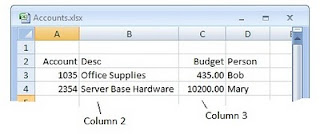
f. Finally, type a comma-",False", which tells the formula it must find an Exact-match in the lookup table; this is the most common option.
g. Close the parenthesis) and press Enter. The completed formula:
=Vlookup
(B5,[Accounts.xlsx]MasterAccounts!MyAccounts,2,False)
=Vlookup(B5, [Accounts.xlsx]Sheet1! MyAccounts,2,False)
Results: The Description for account code 2356 ("Networking") is returned.
Lookup another Column in the same Table
In cell D5, one cell to the right, build another VLookup formula, returning the budget amount:
=VLookup (B5,Accounts.xlsx!MyAccounts,3,False)
where:
- Accounts.xlsx is the name of the sheet
- "MyAccounts" is the name of the named-range
- "3" returns the budget from the third column
- "False" means find an exact match
Improved VLookup Formula:
There is a possibility the Vlookup may not find a given account-code; usually because of a mis-keyed value or the account does not exist. Test this now by doing the following:
a. In the original cell B5 ("2356"), change the account code to a non-existent account ("2000"). Results: The Vlookup formulas return "#N/A" (Value not found).
Improve the Formula using IFError:
b. Cosmetically, this can be improved with this formula in Cell C5 (all on one line):
IfError(VLookup(B5,Accounts.xlsx! MyAccounts,2,False),"Not Found")
c. In D5, use this formula (note the double-quotes ""):
IfError(VLookup(B5,Accounts.xlsx! MyAccounts,3,False),"")
where:
- =ifError says if "any part of the included formula generates any kind of error (such as a #N/A"), put a different value in the cell. Otherwise, use the original value.
- Do not use an equal-sign in front of the VLookup clause
- If an error was found, the formula returns the literal text "Not Found".
Cell D5's formula, the second VLookup was changed to return a null (empty) string (quote-quote) if there was an error.
- Depending on your needs, the formulas could also return a zero (0) instead of the text "Not Found".
Possible Errors:
- #N/A (#NA) - An exact match was not found in the lookup table.
- #N/A The lookup cell address may have shifted or changed, confirm the first parameter is pointing at the value you want to lookup.
- #Name? - An incorrect or misspelled RangeName (aka "MyAccounts") or the range-name does not exist.
Range-Name Issues:
If you choose not to use a range name in the VLookup, you will have to use a cell-range.
=Vlookup
(B5,[Accounts.xlsx]MasterAccounts!$A3:D13 ...
where $A3:D13 are all the values typed in the lookup table.
These types of ranges are inherently fragile. If new values are inserted into the lookup table while your original sheet is closed, the lookups will not see the change and the wrong range will be selected, often resulting in "#NA" values.
With explicit addresses (A3:D13), the range may or may not expand when new rows are inserted into the table, depending on which linked sheets were opened at the time. Compare this to a range-named table, where inserted records automatically expand the range-name. In other words, explicit addresses (A3:D13) are risky.
However, with either the RangeName or explicit-address examples, newly-inserted records at the top-most or bottom-most records will not expand the range-names correctly and VLookups will have sporadic failures when they are near these areas. When inserting new values in the lookup on the first or last row, check the range-name to make sure it is still accurate.
Confirming an existing Range-Name:
When inserting records on the top-most or bottom-most rows, confirm the range with one of these methods:
Method 1:
Click the down-doodad right above column A, choose the Range-name "MyAccounts".
Excel will highlight the cells.
Confirm the highlight encompasses all rows and columns.
See below if you need to change.
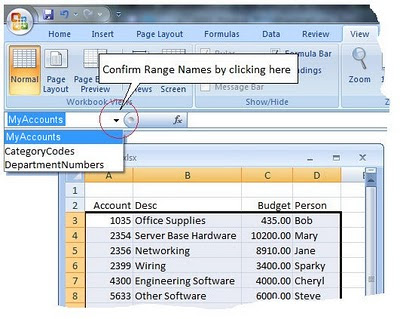
Method 2:
Use this method to check and, if needed, to change the selected range in the Range-name:
In Excel 2007's ribbon menu, choose "Formulas", Name Manager or press Control-F3.
Confirm the range-name cell address (e.g. $A$3:$D$13). The dollar-signs are important for reasons not described here. To change the range-values, click the red-arrow and re-highlight the table. This example shows a sheet with other range-names:
As an aside, you can see all linked sheets (from your main sheet, not from the Accounts Sheet) by selecting the top-menu Data, Edit Links. "Accounts.xlsx" will show as a linked sheet.
Other Range Names
In the lookup-table sheet, where the MyAccounts range lives, you can have other sections devoted to other lookup values. For example, there might be a Department Lookup table, CategoryCodes, Employee lookup, etc. All can live in the same sheet and all will work well if you use Range Names.
Performance Concerns
Vlookups are somewhat expensive in CPU processing. If your sheet has thousands of lookups, the performance of the sheet could be slow. Consider the following to improve the speed:
- Open the lookup sheet *before* opening your main sheet.
- On really large sheets, set manual re-calculation: Menu: Formulas, Calculation Options, Manual. Understand the implications before doing this.
- The lookup sheet can be closed and the formulas will still work; you will be prompted for establishing the link when you open your main sheet.
Dirty Data:
With numeric lookups, occasionally, the lookup key values may look like numbers, but are really textual. This can happen if the table is populated from a mainframe download or other ASCII import.
The symptoms are this: Both the lookup table and the lookup value might show '2356' -- but one is numeric and the other is character. When run through the VLookup, you will get an unexpected "Not Found" or NA.
To test the textual-data, make a dummy formula in another section of the lookup-sheet. Add +1 to your suspected numeric value. If it is text, the answer will be "1"; if numeric it will be '2357'. Do the same for the test value in the vlookup sheet.
If the 'numeric' values in the lookup sheet are really character, correct the issue by converting the lookup column to numeric data. Do this with these steps in the lookup columns:
a. Insert a new dummy column.
b. Use this formula: "=Value(
c. Fill the formula down the column.
d. Copy the formulas; use Paste-Special, Values-only, over the top of the original "numbers".
e. Delete the dummy column.
You may also find the original data is polluted with non-printable characters -- usually a tab. Consider using similar steps with a =Clean() formula to spiff the data.
Non-Exact Searches
The last parameter in the VLookup (,"false"), tells Excel that an exact match must be found. This is the normal setting for the formula. However, you can specify a non-exact match.
For example, if the dollar figures were between $1,000 and $2,000 dollars, use such-and-such General-Ledger number. But if the number were between $2,000 and $10,000, use a different number.
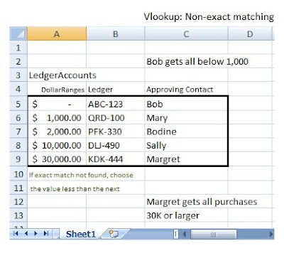
Consider this table, which shows purchase-order approval ledger information:
 Within your own sheet, a lookup of various items purchased, might look like this, where different ledger-numbers and approving people are displayed, depending on the dollar-amount spent:
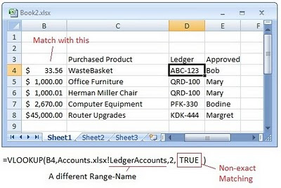
The formula in cell D4 ($33.56 purchase) would look like this:
=VLOOKUP(B4,Accounts.xlsx!LedgerAccounts,2,TRUE)
where:
- "LedgerAccounts" is a new RangeName in the lookup sheet.
- "2" returns the second column (Ledger-account number)
- "true" says allow inexact matches
With this type of lookup, you do not need the IfError logic used in previous examples -- there is no need unless you expect negative numbers to arrive.
In the lookups, Bob (Ledger account ABC) gets to approve all dollar purchases less than $1,000. If the purchase were $1,000.01, Mary gets the right to approve (not Bodine).
All purchases $30,000 or larger belong to Margret. The rule is this: If no exact match is found, find the next larger value that is less-than the looked-up value.
This concludes the VLookup tutorial. Your comments are welcome.
Related Keyliner Articles:
Excel UDF (User Defined Functions)Using Excel for Raffle-Ticket Drawing: Prizeorama
Excel VLookup - a complete tutorial
Excel Coloring Alternate Rows
Excel Parsing City-State-Zip
Excel Importing Text with Leading Zeroes
VB - Return First Word, Last Word, Supertrim
Using VBA to Send Email
Using Excel to select Raffle Tickets - Prize-orama


No comments:
Post a Comment
Comments are moderated and published upon review. (As an aside, not a single spam has been allowed through; why bother?)